Semi-log plot of detected cases (blue)
and deaths (red) from CoVid-19
in the United States --- from the
Wikipedia Covid-19 'pandemic in the United States' page
in early April 2020
(Data Source: World Health Organization)
Simple Math (Arithmetic)
|
(2020 Apr blog post)
SECTIONS BELOW:
INTRO
GROWTH-DECLINE EQUATIONS
COMPUTATION METHOD
DATA TABLES BELOW:
! Note !
Text or web-links or images may be added
(or changed) --- if/when I re-visit this page.
|
INTRODUCTION : In March 2020, I assembled a 'Math-for-Epidemics' web page that shows how any person (including Trump) could come up with 'ball park' estimates for how an epidemic in a given region (and for a given infection or death rate) would grow exponentially. That page includes several numerical computation examples for several different 'infection rates'. The differential equation that codifies that exponential growth was presented ... namely: dx/dt = R * x (DE1) where x is a number representing the count of the number of infected in the population and R is a 'proportionality constant'. The left-hand-side, dx/dt, is a 'rate of change' ratio --- and can be thought of as the 'velocity or speed of the infection'. The right-hand-side gives us a 'law' for determining that rate of change. As an example, R = 2.0 is the case of the 'change of the population' doubling 'off of' the current number of the population --- for each increment of a chosen time step. The symbol 'dt' represents that time step --- and 'dx' represents the change in the infected population count over one instance of that time step. It was pointed out that a suitable time-step for our numerical computations is dt = 1 week. It was also pointed out that, for numerical computation purposes, we could use two simple equations:
dx = R * x(t)
And that pair of equations (involving one multiplication and one addition at each time step) could be simplified to one equation (which would enable us to do just one multiplication at each time step, no addition). Namely: x(i+1) = (1 + R) * x(i) for weeks i = 0, 1, 2, 3, ... This equation was used to generate data tables for several different infection rates --- R = 2.0, 4.0, and 5.0 --- corresponding to infection rates one may see with a very virulent virus such as the Covid-19 virus. However, that computation has a big limitation. Although it allows us to get an idea of the 'initial' exponential growth rate of the infection, it does not provide us a way to model the eventual 'fall off' of the infection as the population of 'susceptibles' declines. It is the intent of this web page to show how any person (including Trump) could come up with 'ball park' estimates for how an epidemic in a given region (and for a given infection rate) would grow --- AND, in addition, model the peak and decline of the infection. SOME DATA SOURCES Like in the 'Simple Math for Epidemics' web page, I will use the following sources of data for determining parameter values for the growth-and-decline equation presented below. Within a month after the coronavirus broke out in China, there were many Wikipedia pages on the '2019' virus --- including pages that showed bar charts of the number of new infections and deaths (a bar for each day) --- for many countries of the world --- and for states (and cities) of the United States. Examples:
I may use data from these Wikipedia pages to eventually try some simulations for several different regions, such as
(We will either assume that the region is essentially 'isolated' --- or we may account for migration of infected people into -- and out of -- the region by an appropriate choice of the rate constant, R.) |
|
MATH FOR INFECTION GROWTH-AND-DECLINE Toward the bottom of the 'Simple Math for Epidemics' web page, it was pointed out that we should be able to fairly accurately model the exponential increase in infections --- AND the eventual decrease in the rate of infection --- by using a 'differential equation' like the following: dx/dt = R * x(t) * (1.0 - x(t)/POP) where x(t) is the number of infected people --- and POP is the total number of people in the region that we are modelling. We are using the fact that the spread of the infection is not only proportional to the number of infected people, x(t) --- but also, the spread is proportional to a measure of the number of 'susceptibles' in the population. The factor (1.0 - x(t)/POP) provides that measure --- where x(t)/POP gives the fraction of the population that is infected --- and (1.0 - x(t)/POP) gives the fraction of the population that is not infected, i.e. 'susceptible'. Let us abbreviate 'x(t)/POP' as 'IRAT' --- the 'Infected Ratio' of the population. And let us abbreviate (1.0 - x(t)/POP) = (1.0 - IRAT) as SRAT -- the 'Susceptible Ratio' of the population. Then we can write the differential equation above more compactly as dx/dt = R * SRAT * x(t) Note that this essentially turns the exponential growth differential equation DE1 dx/dt = R * x(t) where R is a constant into a differential equation dx/dt = (R * SRAT) * x(t) (DE2) where (R * SRAT) is a 'rate factor', but it is no longer a constant. In fact, this 'rate factor' eventually would go to zero when the number of infected reaches the entire population of the region being modelled --- because SRAT would go to zero. Further, note that, initially, when the number of infectives, x(t), is near zero, the factor SRAT = (1.0 - x(t)/POP) is near 1.0. This means that, intitially, the differential equation dx/dt = (R * SRAT) * x(t) (DE2) will generate values of x(t) like those generated by the diffential equation dx/dt = R * x(t) (DE1)
A Note on 'Recoveries' I should point out a 'further complication' of the typical epidemic. Namely, some of the 'infecteds' of the population will start testing 'negative' for the virus. So part of the infected population, x(t), will no longer be infective. Note that the equation DE2 above is meant to say that the number of 'new infections' 'dx' (in a time step) is proportional to the product of factors representing both the number of 'susceptibles' and the number of people still 'shedding' the virus --- not the number of people who have contracted the virus. (This is similar to the 'rate equations' of chemical kinetics where the chemical reaction proceeds at a rate proportional to the product of the population of each of the various chemical molecules. Thus, if a population of one of the molecules declines and goes to zero, the rate of the reaction declines and goes to zero.) So the factor 'x(t)' on the right-hand-side of the DE2 above should be reduced by the amount of 'recoveries' (assuming that a recovered person has built up an immunity and can no longer host the virus and spread the virus). There are various reports that indicate, for a virulent virus like Covid-19, it will take at least 2 weeks --- and probably more like 4 or 5 weeks --- for an infected individual to stop 'shedding' the virus. That 'stopping of shedding' is something that could be taken into consideration by a 'time-delay' term in the equation DE2. In particular, note that x(t) represents the cumulative number of infected people --- which includes the 'recoveries' (non-shedders) as well as those still shedding virus. Let us assume that 'tr' represents the amount of time it takes for an infected person to 'recover' --- and no longer be shedding the virus. (tr = time to recover) Then, at time 't', the cumulative amount x(t - tr) --- the number of 'infecteds' up to time 't - tr' --- is the cumulative number of 'recoveries'. Then (x(t) - x(t - tr)) is the number of 'infecteds' at time 't' that are still shedding the virus. In equation DE2 above: dx/dt = (R * SRAT) * x(t) (DE2) the factor x(t) was supposed to represent the number of people still 'shedding' the virus, and thus causing more infections. But that factor does not take into account the 'recoveries'. We should replace the factor x(t) by the factor (x(t) - x(t - tr)) --- giving us the time-delay differential equation dx/dt = (R * SRAT) * (x(t) - x(t - tr)) (DE3) where x(t) still represents the cumulative number of people, at time 't', that have been infected at some time in the past. For the Covid-19 virus, which is spreading so fast, the major part of the infection process will be over by the time that significant numbers of the infected population, x(t), become non-infective ('recovered'). So we could use equation DE2, rather than DE3, and probably get good results for a majority of the time of the simulation --- until near the end, when the number of 'recoveries' finally become a significant number. Note that in the infected number x(t), it is the infecteds that existed about 4 weeks and more ago, that are no longer infecting people. In an infection where x(t) is tripling every week (like for R=2.0), the people infected 4 weeks ago are a tiny portion of the current population of infectives --- about (1/3)^4 = 1/81 of the current infectives. So, for a very virulent virus, that causes an infected person to remain 'infective' for many weeks, we can expect to get good modelling results with the equation DE2 that we presented above: dx/dt = (R * SRAT) * x(t) (DE2) However, to monitor where in the simulation the factor x(t) is becoming an over-estimate of the number still shedding the virus, we could calculate, at each time step in our simulation tables, the number given by 'x(t) - x(t - tr)' --- which estimates the number of people 'shedding virus' at time 't'.
METHOD OF NUMERICAL COMPUTATION Now, like we did on the 'Simple Math for Epidemics' web page, we will show how we can convert the 'differential equation' DE2 above into equations that we can use for numerical computation. Again, we think of the unknown 'x' as a 'function of time' --- typically denoted 'x(t)'. And we want to generate values for 'x' at various times 't'. To use the 'rate equation' --- dx/dt = R * SRAT * x(t) --- to make numerical predictions, we actually use it in a different form: dx = R * SRAT * x(t) * dt This equation says that the 'change in x' (near a given time 't') is the product of R and SRAT and x(t) and dt. For predictions of growth/change in epidemics, it is typical to use dt = 1 --- such as one week (or one day). So, for computational purposes, we use the simple equation: dx = R * SRAT * x(t) where 'R' must be based on the same time-units as 'dt' --- and SRAT is a 'dimensionless' factor. The equation above gives a number 'dx' representing a change in 'x' near a time 't'. However, that does not give us 'x' at a next time step. For that, we need an additional very simple equation: x(t+dt) = x(t) + dx This equation simply says that the value of 'x' at a 'next time step' is given by the value of 'x' at the 'previous time step' PLUS the change in 'x' that we got from the rate equation: dx = R * SRAT * x(t) STARTING THE COMPUTATION OK. So now we have the two simple equations that we will use to generate x(t) at various times --- t, t + dt, t + 2*dt, t + 3*dt, ... The two simple equations are
dx = R * SRAT * x(t) But now we need a bit of data to start the computation. This bit of data is called an 'initial value' or 'initial condition'. In general, we can think of wanting to generate a table of values of 'x' at times t0, t1, t2, t3, ... And, in our 'constant-time-step' case:
t1 = t0 + dt, where dt = 1 (week, say). Then, to start off our computation, we need a value of 'x' at initial time 't0' --- denoted x(t0). Then we simply start computing, using the pair of equations above, over and over:
dx = R * SRAT * x(t0)
dx = R * SRAT * x(t1)
dx = R * SRAT * x(t2) and so on. For simplicity, we will let t0 = 0. Then as we successively add dt = 1 to t0, we get t1 = 1, t2 = 2, t3 = 3, ... Then, with this 'one unit time step', the pairs of equations above become:
dx = R * SRAT * x(0)
dx = R * SRAT * x(1)
dx = R * SRAT * x(2) and so on. |
|
A PREDICTION BASED ON R=4.0 On the 'Simple Math for Epidemics' web page, I presented exponential growth tables for R = 2.0. 4.0, and 5.0. Let us use the case R = 4.0 for the 'initial growth factor' of the infection. (This is the constant factor, R, that provides the initial exponential growth of 'x' in the simulation. And it can be determined from data in the early stage of an epidemic. An example of such a determination is seen at the graph below.) In this 'growth-and-decline' model, that constant factor, R, is modified by the factor SRAT = (1.0 - x(t)/POP). So we have the constant parameter POP to determine. Let us model the entire United States as one 'lumped' region --- so that POP is about 330 million people. Admittedly, the Covid-19 virus is 'rolling out' to different regions of the United States with their own parameters, R and POP. Later, we can try modelling a sub-region of the U.S.--- such as the 'metropolitan area' of New York City --- or a state such as South Dakota or Louisiana or Florida or Missouri (assuming the population of those regions is essentially constant and that most of the 'later' infections are being transmitted from the residents of the region and not from travellers/migrants). The following table is one that I generated based on the fact that, in mid-March 2020, there were said to be about 5,000 reported cases of infections, in the United States, from the 2019-coronavirus (Covid-19). In this case, our 'x(t)' will denote the number of total reported Covid-19 infections at time 't' --- in the United States. Note that at week-zero, we start with the value x(0) = 5K.
At each time step i = 1, 2, 3, ...,
We will also present a column for estimated number of deaths, by using a rough estimate for the Covid-19 virus of one-percent of the cumulative number of infected, x(i). To monitor an estimated number of 'recoveries', we will also present a column for (x(i) - x(i-4)), where we are assuming 4-weeks for recovery. |
   ----------------------------------------------------------
   Virus Infection Simulation
   ( R = 4.0 times per week ; i.e. quadrupling 'dx', initially)
   ( POP = 330 million = 330,000K)
                                                                                                                                    Cumulative
  End of    IRAT         SRAT           Added                 Cumulative                                                         Infecteds minus Recoveries
   Week   (x(i-1)      (1.0 -        Infections             Total Infections                        Cumulative Total Deaths      (Current 'Virus Shedders')
  Number    /POP)        IRAT)   (dx = R*SRAT*x(i-1))     ( x(i) = x(i-1) + dx )                    (1% of Cum. Infections)      ( x(i) - x(i-4) )
  ------ -----------   ----------  ---------------------  ----------------------                    -------------------          -------------------
    0                                                       5K                     mid-March         50                           ? somewhat less than 5K
    1      1.5e-5       ~1.0     4*1.0*5K = 20K             5K +     20K = 25K                       250                          ? somewhat less than 25K
    2      7.5e-5       ~1.0     4*1.0*25K = 100K           25K +   100K = 125K                      1250                         ? somewhat less than 125K
    3      .00037       ~1.0     4*1.0*125K = 500K          125K +  500K = 625K                      6250                         ? somewhat less than 625K
    4      .0019        .998     4*.998*625K = 2495K        625K + 2495K = 3120K     mid-April       31,200                       3,120K - 5K = 3,115K  (-0.16%)
    5      .0095        .990     4*.990*3120K = 12355K      3120K + 12355K = 15475K                  154,750                      15,475K - 25K = 15,450K (-0.16%)
    6      .0469        .953     4*.953*15475K = 58990K     15475K + 58990K = 74465K                 744,650                      74,465K - 625K = 73,840K (-0.8%)
    7      .2257        .774     4*.774*74465K = 230543K    74465K + 230543K = 305008K               3,050,080                    305,008K - 3120K = 301,888K (-1.0%)
    8      .9243        .0757    4*.0757*305008K = 92356K   305008K + 92356K = 397364K   mid-May

                                                            330000K = U.S. population
                                                            The simulation stops here
                                                            --- between weeks 7 and 8
                                                            --- just before mid-May.
|
Note that the value of x(i) --- cumulative infections --- for the first several weeks matches the results that we saw for the R=4.0 table on the 'Simple Math for Epidemics' web page --- for simple exponential growth, without limits. Suddenly, between weeks 6 and 7, the number of 'susceptibles' changes from about 95% to about 77% --- so the multiplication factor (R * SRAT) becomes about 4.0 * 0.77 = 3.08 instead of 4.0. Between weeks 7 and 8, the 'new infections, weekly' (dx) finally peak and go down from about 230 million to about 92 million. Actually, between weeks 7 and 8 (just before mid-May), the simulation would stop because the entire U.S. population will have experienced infection --- and, if this virus behaves like most previous viruses, 'herd immunity' will have been achieved. DEATH PREDICTIONS Some of the initial data from the United States indicated that the number of deaths (from Covid-19) was about one percent of the number infected. Using that fact (rough estimate), we see (on the right in the table above) that the number of deaths in the United States from Covid-19 may be on the order of 31,000 by mid-April 2020. And, just before mid-May 2020, when 'herd immunity' is acheived (as essentially the entire population becomes infected), the number of deaths may 'plateau' at about 3 million.
Note that this 3 million figure would be predicted simply by observing that then one-percent of 330 million gives us approximately 3 million deaths, eventually. If it turns out that about ONE-TENTH-OF-ONE-PERCENT of 'infecteds' dies (like the death rate from some other corona viruses), then the eventual number of deaths in the U.S. may be about 300,000. EFFECT OF RECOVERIES The column that shows ( x(i) - x(i-4) ) --- the cumulative infecteds minus the cumulative recoveries --- indicates that the time delay of 4 weeks for recoveries means that --- even near the end of the course of the infections --- the recoveries are less than 1 percent of the cumulative infecteds. So, near the end, about 99% of the infecteds are still shedding virus. This is because about 99% of those infecteds were infected in the past 4 weeks and are still 'shedding' virus. That 99% has not had time to recover yet.
Bottom line: However, it may be instructive to re-do this simulation using R=2.0 and equation 'DE3' --- especially since the graph below suggests that the rate of infection in the United States was reduced from about R=3.6 to about R=2.0 --- probably because the New York area was dominating the statistics in March 2020, and New York started observing 'shelter in place' and 'social distancing' pretty thoroughly and consistently. In this situation of 'flattening the curve', it may be the case that if we use the time-delay factor ( x(i) - x(i-4) ) --- instead of x(i) --- there may be an observable effect near the end of the course of the infection. A CRITIQUE OF THE SIMULATION ABOVE The main criticism that could (and should) be levelled at the above simulation is that the United States is not a 'homogeneous' population. Various regions of the country will have different infection rates --- for example, because some parts of the country (like Florida) did not practice 'social distancing' (of 'residents' nor of 'migrants') to any significant degree. So the infection rate (R) for Florida will probably be much higher than for areas of the country like Northern California (esp. San Francisco) and Southern California (esp. Los Angeles) where the mayors and governor were more pro-active.
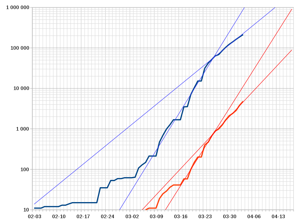
Another example of 'non-homogeneity': Criticism/Observation 2: Another factor to consider in doing infection-simulations like these is that it may not be appropriate to say that the factor R can be considered to be a constant --- and get good predictive results. For example, there are signs that the infection rate in the United States took a rather sudden change --- from one (essentially) constant rate in March 5 to March 25 --- to a lower (essentially) constant rate after March 25 --- probably due to a change to much more rigorous 'social distancing' and 'shelter in place'. See the blue lines in the following graph. |
Semi-log plot of detected cases (blue)
and deaths (red) from CoVid-19
in the United States --- from the
Wikipedia Covid-19 'pandemic in the United States' page
in early April 2020
(Data Source: World Health Organization)
|
Not surprisingly, the 'deaths' curve (red) 'lags' the 'infecteds' curve (blue) by about 14 days, because it is about 14 days after an initial infection that a 'victim' becomes seriously ill. Let us try to get a value for R (a weekly infection rate constant) for the two linear sections of the 'detected cases' blue lines. For the week-long period from March 16 to March 23, we can determine (like we did on the 'Simple Math for Epidemics' web page) that
R = dx / x = (x(i+1) - x(i)) / x(i) =
For the week-long period from March 26 to April 2, we can determine that
R = (180,000 - 60,000) / 60,000 = This kind of change in R could be handled in data tables (like the one above) by switching from one R value to another at an appropriate point in computing the rows of a table. Criticism/Observation 3: Because the simulation above 'blew up' (from thousands to tens of millions of 'infecteds') in weeks 5-6-7-and-8, it would probably be better to perform the simulation with a time-step of '1 day' rather than '1 week' --- at least starting about week 4, if not in the entire table --- in order to see the huge changes occuring within those later weeks. But that would require a lot more computations --- and it would be better to computerize the computations in order be able to generate the table 'in a flash' --- and to experiment with many more values of parameters like R and x(0) and POP. For example, the Tcl-Tk scripting language could be used to present a GUI by which to generate the data and plot it (for values of R and x(0) and POP entered on the GUI). An example (GUI and script) can be seen on a web page that presents a 'tkGooie' script for simulating population growth. Note that switching from weeks to days during the generation of a 'simulation table' would require a switch from a 'per-week' rate constant R to a 'per-day' rate constant. If we computerize the computation, we may as well simply do the entire simulation with a time-step of '1 day' rather than '1 week' --- and require the rate constant R on the GUI to be provided based on a 'per-day' rate, rather than a 'per-week' rate. R-daily and R-weekly: If we have a value of 'R' to use for a 'per-week' simulation (say 'Rw'), we might want to do a 'per-day' simulation --- in which case, we would need to find an 'equivalent' value of 'R' to use for a 'per-day' simulation (say 'Rd'). These values of R are typically determined from data during the initial 'exponential growth' phase of an epidemic. Then these values of R can be used to solve the equation (DE1) above --- to simulate the initial phase of the infection. Recall that we could solve equation (DE1) numerically with the formula: x(i+1) = (1 + R) * x(i) for time-steps i = 0, 1, 2, 3, ... Let us use Xw(i) to represent the values that we would generate with weekly time steps --- and use Xd(i) to represent the values that we would generate with daily time steps. Then the values of Xw(i) could be generated with Xw(i+1) = (1 + Rw) * Xw(i) for weeks i = 0, 1, 2, 3, ... And the values of Xd(i) could be generated with Xd(j+1) = (1 + Rd) * Xd(j) for days j = 0, 1, 2, 3, ... Then we could find the relationship between Rw and Rd as follows --- namely, the relationship: Rw = (1 + Rd)^7 - 1 Let Xw(i) represent the value of Xw at the end of week 'i', which is, say, March 14, for example. Then Xw(i+1) represents the value of Xw at the end of week 'i+1', which would be March 21 in our example. Then let Xd(j) be the value of Xd at the end of day 'j', which is March 14 --- the same day as the end of week 'i'. Let us imagine the two 'time-series' of data --- Xw(i) and Xd(j). There are seven Xd(j) data points for every one data point of Xw(i). And we shall expect that if we start these time-series on the same day with the same initial value, every 7th value of Xd(j) should be equal to every single corresponding value of Xw(i). So in our example above --- we let i and j represent the same day, say March 14 --- then 7 days later, the value Xw(i+1) should equal Xd(j+7). Symbolically we have:
Xw(i) = Xd(j) at the beginning and end of the week --- say, March 14 and March 21. But Xw(i+1) is given by Xw(i+1) = (1 + Rw) * Xw(i) And Xd(j+7) is given by applying the formula Xd(j+1) = (1 + Rd) * Xd(j) seven times. Here is how we would apply that formula 7 times. Xd(j+1) = (1 + Rd) * Xd(j) Xd(j+2) = (1 + Rd) * Xd(j+1) = (1 + Rd)^2 * Xd(j) Xd(j+3) = (1 + Rd) * Xd(j+2) = (1 + Rd)^3 * Xd(j) Xd(j+4) = (1 + Rd) * Xd(j+3) = (1 + Rd)^4 * Xd(j) Xd(j+5) = (1 + Rd) * Xd(j+4) = (1 + Rd)^5 * Xd(j) Xd(j+6) = (1 + Rd) * Xd(j+5) = (1 + Rd)^6 * Xd(j) Xd(j+7) = (1 + Rd) * Xd(j+6) = (1 + Rd)^7 * Xd(j) where '^' represents exponentiation.
(Trump would say--- in his own unique way ---
if he could pronounce 'exponentiation': Then, since we have two different ways of evaluating Xw(i+1): Xw(i+1) = Xd(j+7) = (1 + Rd)^7 * Xd(j) and Xw(i+1) = (1 + Rw) * Xw(i) We can equate (1 + Rw) * Xw(i) = (1 + Rd)^7 * Xd(j) But Xw(i) = Xd(j) on our start date, March 14. So we can cancel (divide by) those equal factors and get (1 + Rw) = (1 + Rd)^7 This gives us our relationship between Rw and Rd. We can rearrange this to give Rw in terms of Rd --- namely: Rw = (1 + Rd)^7 - 1 Using this relationship, we can build a data table (like the following) relating Rd and Rw for representative useful values --- for doing simulations of virulent virus infections. Using a 'scientific calculator' with an 'x^y' key, the following table was built.
So, for example, when we used Rw = 2.0 to do an infection simulation with a 'per-week' time step (like the R=2.0 data-table below), we could use a value of about Rd = 0.17 to do the simulation with a 'per-day' time step. And when we used Rw = 4.0 to do an infection simulation with a 'per-week' time step (like the R=4.0 data-table above), we could use a value of about Rd = 0.26 to do the simulation with a 'per-day' time step. And if we used Rw = 5.0 to do an infection simulation with a 'per-week' time step (for a very virulent virus infection with no 'social distancing' and 'no shelter in place'), we could use a value of about Rd = 0.29 to do the simulation with a 'per-day' time step. We could also provide a formula for Rd in terms of Rw --- by using logarithm and exponential functions/operators. In most programming languages, there are 'log' and 'exp' functions that can be used to perform those two operations (with the base 'e' = 2.71828... --- the so-called 'natural number', because it arises naturally, for example, when taking compound-interest calculations to 'the limit'.). And on some scientific calculators, there are 'log' and exponential function keys to perform those two operations (with the base 10). We could apply the 'log' function to the relationship above (1 + Rw) = (1 + Rd)^7 to get log(1 + Rw) = 7 * log(1 + Rd) We want to get Rd on one side of the equation, by itself. Rearranging gives log(1 + Rw)/7 = log(1 + Rd) Applying the 'exp' function to each side gives exp(log(1 + Rw)/7) = 1 + Rd Subracting one from each side gives
Rd = exp(log(1 + Rw)/7) - 1
We could use a scientific calculator (or a computer program) to build a table using this formula. This equation could be used to give a very accurate value of Rd for a given value of Rw. But the table above should be accurate enough --- considering all the complicating factors in doing an infection simulation. Criticism/Observation 4: It is natural for people to say that the 'number of infecteds' data being used for these simulations under-reports the number of infecteds because not everyone is being tested. The ACTUAL 'number of infecteds' may be 2 or 3 times --- or even 10 times --- more than the REPORTED 'number of infecteds'. Of the 3 parameters (R, x(0), POP) in the computations above, the typical person will say that both R and x(0) should be larger values. I would like to point out that, indeed, we should probably use a larger value of x(0) --- the 'initial value' --- in the computations above. However, I point out that the way that we determined R is still valid, even though the data may be 'under-reported' by a significant amount. The argument goes as follows. We used the equation R = dx / x = (x(i+1) - x(i)) / x(i) above to determine an appropriate value(s) of R from the semi-log plot above. Let us say that the values of x(i) (in the graph above) are under-reported by a factor N (which could be huge --- 10 or even 100). Then (N*x(i+1) - N*x(i)) / N*x(i) would be used to calculate R. But the N's cancel, and we get the same result as when we used the 'under-reported' values to calculate R with (x(i+1) - x(i)) / x(i) Admittedly, this leaves us with the fact that the initial value, x(0), that we used in simulation above should be much larger. If we re-did the simulation above with a larger x(0), we would find we would end the simulation sooner --- and we would hit the 'apex' of 'dx' and the 'levelling off' of 'x' sooner. |
|
A PREDICTION BASED ON R=2.0 We mentioned above (after the R=4.0 computation with DE2) that it would probably be useful to perform the computation with R=2.0 --- which seems to correspond to 'social distancing' and 'shelter in place' for the Covid-19 virus. At the same time, let us use DE3 (rather than DE2) to take into account the 'recoveries' from infection. In equation DE3, we use the factor (x(i) - x(i-4)) --- instead of the x(i) factor of DE2 --- to take into account that some of the 'past infecteds' are no longer 'shedding virus'. Again, let us model the entire United States as one 'lumped' region --- so that POP is about 330 million people. From the semi-log plot above, we see that there were about 60,000 'REPORTED' cases of infection at about 21 March 2020 (the end of the 3rd week of March). However, the ACTUAL' number of cases of infection may have been several times higher. So we will use 180,000 as our 'initial value' (at the end of the 3rd week of March) --- out of the total U.S. population of about 330 million. In early April 2020, there was a report from Germany that some rather thorough testing of the population of a region in Germany revealed that the number of 'infecteds' of the 'tested' cases in the region were about 3 times higher than the cases that had been 'reported' for the region based on limited testing (mostly of people had been hospitalized or showed definite symptoms). It could be the case that in the United States that the 'under-reporting' is much higher --- but, for the data table below --- we will use a factor of 3 to adjust the 'reported' cases to 'actual' cases --- for our 'initial value' at the end of the 3rd week of March in the U.S. In this 'computation run', the symbol 'x(t)' will denote the cumulative number of 'ACTUAL' Covid-19 infections at time 't' --- in the entire United States. Note that at the end of week-zero, we start with the value x(0) = 3 * 60K = 180K.
At each time step i = 1, 2, 3, ...,
We will also present a column for estimated number of deaths, by using a rough estimate for the Covid-19 virus of one-percent of the cumulative number of infected, x(i). Note that we have replaced the factor x(i-1) of DE2 by the factor (x(i-1) - x(i-5)), where we are assuming 4-weeks for recovery. For the first 4 weeks of the simulation, we do not have values for the number of 'recoveries' x(i-5). We have x(5-5) = x(0), but not x(1-5), x(2-5), x(3-5), and x(4-5). As a rough estimate for those 'recovery figures', we will assume that (since the infecteds, x(i), is roughly doubling to tripling each week), the value of x(i) 4 weeks previous is about (1/2)^4 to (1/3)^4 of x(i). This would mean that the recoveries would be between 6.25% and 1.23% of x(i). We will take the optimistic view that about 6% are recovering each week. |
   ----------------------------------------------------------
   Virus Infection Simulation
   ( R = 2.0 times per week ; i.e. doubling 'dx', initially)
   ( POP = 330 million = 330,000K)

                                    Cumulative
  End of    IRAT        SRAT   Infecteds Minus Recoveries         Added                  Cumulative
   Week   (x(i-1)     (1.0 -   (Current 'Virus Shedders')      Infections              Total Infections                      Cumulative Total Deaths
  Number    /POP)       IRAT)  ( IMR = x(i-1) - x(i-5) )     (dx = R*SRAT*IMR)        ( x(i) = x(i-1) + dx )                  (1% of Cum. Infections)
  ------ -----------  -------  --------------------------  -------------------------  ----------------------                 ---------------------
    0                                                                                  180K                     21March         1,800
    1      .000545     ~1.0     ? about 6% less than 180K   2*1.0*169K = 338K          180K +  338K = 518K                      5,180
    2      .00157      .998     ? about 6% less than 518K   2*.998*487K = 972K         518K +  972K = 1490K                     14,900
    3      .00452      .995     ? about 6% less than 1490K  2*.995*1400K = 2786K       1490K + 2786K = 4276K                    42,760
    4      .01296      .987     ? about 6% less than 4276K  2*.987*4019K = 7933K       4276K + 7933K = 12209K    21April        122,090
    5      .03700      .963     12209K - 180K = 12029K      2*.963*12029K = 23168K     12209K + 23168K = 35377K                 353,770
    6      .1072       .893     35,377K - 518K = 34,859K    2*.893*34859K = 62258K     35377K + 62258K = 97635K                 976,350
    7      .2959       .704     97,635K - 1490K = 96,145K   2*.704*96145K = 135372K    97635K + 135372K = 233007K               2,330,070
    8      .7061       .294     233,007K - 4276K = 228,731K 2*.294*228731K = 134493K   233007K + 134493K = 367500K   21May      ~3 million

                                                                                               330000K = U.S. population
                                                                                               The simulation stops here
                                                                                               --- between weeks 7 and 8
                                                                                               --- around the 3rd week of May.
|
Note that the value of x(i) --- cumulative infections (column 6) --- almost triple each week. This is like we saw for the R=2.0 table on the 'Simple Math for Epidemics' web page --- for simple (initial) exponential growth, without taking into account diminishing numbers of 'susceptibles' --- and increasing numbers of 'recoveries'. This 'tripling trend' continues for about 6 weeks. Then, between weeks 6 and 7, the number of 'susceptibles' changes from about 89% to about 70% --- so the multiplication factor (R * SRAT) becomes about 2.0 * 0.70 = 1.40 --- instead of 2.0 initially. Then, between weeks 7 and 8, the number of 'susceptibles' changes from about 70% to about 24% --- so the multiplication factor (R * SRAT) becomes about 2.0 * 0.24 = 0.48. Between weeks 7 and 8, the 'new infections, weekly' (dx) finally peak and go down from about 135 million to about 134 million. Note that the 'new infections' in weeks 7 and 8 are about one-third (each week) of the population POP = 330 million. So about two-thirds of the infections occur in the last two weeks --- and about one-third of the infections occur in all of the previous weeks, which are about 2 months (8 weeks) more than the first 6 weeks in the table above --- about 14 weeks in all. (Since the Covid-19 infections in the United States probably started around mid-January --- about one-third of the infections 'dribbled on' for about 14 weeks --- mid-January to the beginning of May --- before exploding in about 2 weeks --- according to this 'simulation'.) Between weeks 7 and 8 (around the 3rd week of May), the simulation would stop because the entire U.S. population will have experienced infection --- and, if this Covid-19 virus behaves like most previous viruses, 'herd immunity' will have been achieved. It should be pointed out that epidemiologists say that 'herd immunity' may be reached when about 70% of the population becomes infected. Since 0.7 x 330 million is about 231 million, the table above indicates that the infections may effectively stop at about week 7 (mid-May) --- when about 233 million infections are predicted. Of course, these are rough calculations that do not take into account that there may be 'hermit-like' pockets of people in the United States that do not come into contact with 'infecteds' for many months. ALSO, about half the population of the U.S. started practicing 'shelter in place', 'social distancing', and 'mask wearing' around mid-April. This would probably result in the infection rate R=2.0 being much too high. A better simulation could be one that models the U.S. as two or three 'compartments' with different infection rates --- such as 'urban' and 'rural' compartments --- OR 'urban-distancing', 'urban-TheVirusCantHurtMe', and 'rural'. So the infections may 'dribble on' for many months in the United States --- as the infections have dribbled on --- even, to a small extent, in countries with aggressive testing-tracing-quarantining programs --- such as South Korea and Singapore. As has been pointed out by various health officials (and non-officials such as Bill Gates), there will probably be continued cases and perhaps another outbreak in the fall of 2020 --- until there is an effective vaccine for the Covid-19 virus.
At the third week of May 2020, the infection cases and deaths in Brazil were skyrocketing --- and there was very little social-distancing and mask-wearing being practiced. The 'aggressive' simulations above --- for R=4.0 and R=2.0 --- may provide a reasonably good predictor of what may happen to a major part of the population of Brazil (about 210 million) --- in terms of shape of the curve and the time interval to massive infection. Other Observations It is easy to make math errors in doing these calculations manually. So it would be really helpful to computerize these calculations as noted above, after the R=4.0 table. Furthermore, it would be helpful to do the calculations 'per-day' rather than 'per-week' --- to see more clearly what is happening in weeks 6 through 8. As indicated above at 'Criticism/Observation 3', I may someday make a Tcl-Tk script --- that presents a GUI in which to enter parameters like R and x(0) and POP --- to do the calculations (and a plot) in a fraction of a second. I would probably alter a 'tkGooie' script for simulating population growth --- to make calculations 'infinitely' faster --- and to eliminate the 'error-prone-ness' of manual calculations. The script could even accomodate a multi-compartment model with, say, 3 compartments, with different infection rates and populations --- and 3 different 'intial values' at a common simulation-start time.
TO BE CONTINUED At this point, I pause to publish this page as-is. In coming days, I may provide
Since this page has become quite long, I would present the additional 'numerical experiments' on a separate web page. More later --- perhaps. |
|
For further information : In case I do not return to update this page, here are a few keyword WEB SEARCHES that you can use to provide updates. |
|
Bottom of this page on
To return to a previously visited web page location, click on
the Back button of your web browser, a sufficient number of times.
OR, use the History-list option of your web browser.
< Go to Top of Page, above. >Or you can scroll up, to the top of this page. Page history:
Page was created 2020 Apr 03.
|